Mathematica

Mathematica is a computational software program used in many scientific, engineering, mathematical and computing fields. It was conceived by Stephen Wolfram and is developed by Wolfram Research of Champaign, Illinois. Mathematica is renowned as the world’s ultimate application for computations. But it’s much more—it’s the only development platform fully integrating computation into complete workflows, moving you seamlessly from initial ideas all the way to deployed individual or enterprise solutions.

Usage #

In order to access the executables load one of the modules, e.g.:

module add math/Mathematica

For interactive computing on the login nodes (testing only) start Mathematica. Scripts can be executed with math.

See the vendor documentation for more detail. For a primer on parallelization with Mathematica we recommend this part of the documentation.

Submitting Jobs: Things to consider #

You may for example submit a mathmatica script with the following command line:

srun -n x --mem=xxx -p short --time <sometime> math -script <path to script>

where

• x reflects the number of wanted cores ( 1 <= x < 64 ; see below on how to retrieve this number within a script)
• xxx the amount of memory required for the job (see the memory reservation page for hints)
• sometime the required wall clock time
• should indeed be a valid path (relative paths should work, too)

Interactive Usage #

Using Mathematica interactively can be done like for any other graphical user interface with interactive jobs using salloc.

SLURM specific Snippets #

In order to retrieve the JobID, you can do

JOBID = Environment["SLURM_JOB_ID"];

The job directory therefore becomes

LocalScratchDir = "/localscratch/"<>JOBID<>"/";

A ramdisk can be reserved as described in this link (broken link, page does not exist anymore). The number of reserved cores can be retrieved with

CPUn = ToExpression[Environment["SLURM_JOB_CPUS_PER_NODE"]];
Print["Number of Processes: "<>ToString[CPUn]];

Submitting a Serial Mathematica Job #

We want to write a one-line example of a Mathematica job to show how it can be executed on our servers.

For that we use the typical Hello MOGON! example

Print["Hello MOGON!"]

It needs to be saved using the extension .wls

#!/bin/bash
#SBATCH --partition=smp
#SBATCH --account=<Your JGU-Account>
#SBATCH --time=0-00:01:00
#SBATCH --mem=512 #0.5GB
#SBATCH --ntasks=1
#SBATCH --job-name=math_serial_example
#SBATCH --output=%x_%j.out
#SBATCH --error=%x_%j.err

module purge
module load math/Mathematica

math -script hello_mogon.wls

The start-up option script is needed, that way Mathematica knows that it should run the file given in the option.

Now the job is submitted with the following command

sbatch serial_math_job.slurm

After the job completes, you can view the output with:

cat math_serial_example_*.out

which should give you

Hello MOGON!

Submitting a Parallel Mathematica Job #

The Wolfram Language uses independent kernels as parallel processors. It is clear that these kernels do not share a common memory, even if they happen to reside on the same machine. However, the Wolfram Language provides functions that implement virtual shared memory for these remote kernels.

Mathematica Documentation, Virtual Shared Memory

So by default Mathematica uses distributed processing, which means that memory isn’t shared.

ParallelDo[
    Print["Hello MOGON! The number of iteration is ",i," from Thread ",$KernelID,"/",$KernelCount],{i,10}
];

#!/bin/bash
#SBATCH --partition=smp
#SBATCH --account=<Your JGU-Account>
#SBATCH --time=0-00:02:00
#SBATCH --mem-per-cpu=1024 #1GB
#SBATCH --nodes=1
#SBATCH --ntasks-per-node=1
#SBATCH --cpus-per-task=6
#SBATCH --job-name=smp_math
#SBATCH --output=%x_%j.out
#SBATCH --error=%x_%j.err

module purge
module load math/Mathematica

math -script hello_mogon_smp.wls

Once the job is finished, you can display the result with the following command:

cat smp_math_*

The output should be similar to the following lines:

From KernelObject[6, Local kernel]:
Hello MOGON! The number of iteration is 1 from Thread6/6

From KernelObject[5, Local kernel]:
Hello MOGON! The number of iteration is 3 from Thread5/6

From KernelObject[4, Local kernel]:
Hello MOGON! The number of iteration is 5 from Thread4/6

From KernelObject[3, Local kernel]:
Hello MOGON! The number of iteration is 7 from Thread3/6

From KernelObject[2, Local kernel]:
Hello MOGON! The number of iteration is 9 from Thread2/6

From KernelObject[1, Local kernel]:
Hello MOGON! The number of iteration is 10 from Thread1/6

From KernelObject[6, Local kernel]:
Hello MOGON! The number of iteration is 2 from Thread6/6

From KernelObject[5, Local kernel]:
Hello MOGON! The number of iteration is 4 from Thread5/6

From KernelObject[4, Local kernel]:
Hello MOGON! The number of iteration is 6 from Thread4/6

From KernelObject[3, Local kernel]:
Hello MOGON! The number of iteration is 8 from Thread3/6

Submitting a Mathematica GPU Job #

Before you start parallelising with Mathematica on MOGON GPUs, you need to prepare your Mathematica environment for the usage of GPUs. Your slurm script needs this command (and the SBATCH options should be configured as for any GPU job)

module load system/CUDA

and you need this command in your script

Needs["CUDALink`"]

You can check whether it works with

Print["Using a ", CUDAInformation[1,"Name"]]

which should for example return

Using a NVIDIA GeForce GTX 1080 Ti

CPU/GPU Bandwidth #

The test estimates how fast data can be sent to and read from the GPU. However, there is also some overhead included in the measurements, in particular the overhead for function calls and array allocation time. Because those are present in any “real” use of the GPU, it is reasonable to include them. Memory is allocated and data is sent to the GPU using CUDAMemoryLoad[]. Memory is allocated and data is transferred back to CPU memory using CUDAMemoryGet[].

The theoretical bandwidth per lane for PCIe 3.0 is $0.985 GB/s$. For the GTX 1080Ti (PCIe3 x16) used in our MOGON GPU nodes the 16-lane slot could theoretical give $15.754 GB/s$.(( This example was taken from the MATLAB Help Center and adapted.))

#!/usr/bin/env wolframscript
Needs["CUDALink`"]

Print["Using a ", CUDAInformation[1,"Name"]]

sizes = Power[2, Range[10, 30, 2]]

mmTimesHost = Range[Length[sizes]]
mmTimesGPU = Range[Length[sizes]]

For[i=1,i<=Dimensions[sizes][[1]],i++,

    Print["Calculating ", sizes[[i]]/8, "x", 1];

    A = RandomInteger[{0,9},sizes[[i]]/8];
    timing = AbsoluteTiming[CA = CUDAMemoryLoad[A];];
    mmTimesGPU[[i]] = {sizes[[i]], sizes[[i]]/timing[[1]]/10^9};

    Print["To GPU time: ", timing[[1]], "s, bandwith: ", mmTimesGPU[[i]][[2]]];

    timing = AbsoluteTiming[CUDAMemoryGet[CA];];
    mmTimesHost[[i]] = {sizes[[i]], sizes[[i]]/timing[[1]]/10^9};

    Print["From GPU time: ", timing[[1]], "s, bandwith: ", mmTimesHost[[i]][[2]]];

]
myTicks = Table[{10^i, Superscript[10, i]}, {i, -20, 15}]

Export["combined_transfer_" <> ToString[UnixTime[]] <> ".pdf",
    ListLogLinearPlot[ Table[{mmTimesGPU, mmTimesHost}], Ticks -> {myTicks, Automatic},
    Joined -> True,
    AxesLabel -> {"Matrix elements ", "Transfer speed (GB/s)"},
    PlotLabel -> "Data transfer",
    PlotLegends -> {"Send to GPU", "Gather from GPU"}]]

The job script is pretty ordinary. In this example, we use only one GPU and start Mathematica with four threads. To do this, we request one process with four cpus for multithreading:

#!/bin/bash
#SBATCH --account=<Your JGU-Account>
#SBATCH --job-name=gpu_transfer
#SBATCH --output=%x_%j.out
#SBATCH --error=%x_%j.err
#SBATCH --partition=m2_gpu
#SBATCH --gres=gpu:1
#SBATCH --time=0-00:10:00
#SBATCH --mem=11550
#SBATCH --ntasks=1
#SBATCH --cpus-per-task=4

module purge
module load system/CUDA/
module load math/Mathematica

math -script gpu_transfer_perf.wls

The job is submitted with the following command

sbatch math_gpu_transfer_job.slurm

The job will be finished after a few minutes, you can view the output as follows:

cat gpu_transfer*.out

The output should be similar to the following lines:

Using a NVIDIA GeForce GTX 1080 Ti
Calculating 128x1
To GPU time: 0.238286s, bandwith: 4.297356957605566*^-6
From GPU time: 0.000191s, bandwith: 0.005361256544502618
Calculating 512x1
To GPU time: 0.000226s, bandwith: 0.018123893805309738
From GPU time: 0.000114s, bandwith: 0.035929824561403506
Calculating 2048x1
To GPU time: 0.000186s, bandwith: 0.08808602150537637
From GPU time: 0.000115s, bandwith: 0.14246956521739132
Calculating 8192x1
To GPU time: 0.000313s, bandwith: 0.20938019169329072
From GPU time: 0.000196s, bandwith: 0.33436734693877557
Calculating 32768x1
To GPU time: 0.000299s, bandwith: 0.8767357859531772
From GPU time: 0.000179s, bandwith: 1.4644916201117322
Calculating 131072x1
To GPU time: 0.000337s, bandwith: 3.1115014836795254
From GPU time: 0.00022s, bandwith: 4.7662545454545455
Calculating 524288x1
To GPU time: 0.000477s, bandwith: 8.793090146750526
From GPU time: 0.000369s, bandwith: 11.366677506775067
Calculating 2097152x1
To GPU time: 0.004637s, bandwith: 3.6181186111710164
From GPU time: 0.003934s, bandwith: 4.264671072699543
Calculating 8388608x1
To GPU time: 0.015336s, bandwith: 4.37590401669275
From GPU time: 0.014839s, bandwith: 4.522465395242267
Calculating 33554432x1
To GPU time: 0.05792s, bandwith: 4.634590055248619
From GPU time: 0.058762s, bandwith: 4.568181069398591
Calculating 134217728x1
To GPU time: 0.233188s, bandwith: 4.604618693929361
From GPU time: 0.232933s, bandwith: 4.6096595329987595

The script also generates a plot, which we would like to show here:

Memory Intensive Operations #

You might be familiar with this example if you stumbled upon our MATLAB article or read it on purpose. At this point we would like to restate what we originally took from the MATLAB Help Center:

For operations where the number of floating-point computations performed per element read from or written to memory is high, the memory speed is much less important. In this case the number and speed of the floating-point units is the limiting factor. These operations are said to have high "computational density".

A good test of computational performance is a matrix-matrix multiply. For multiplying two $N
times N$ matrices, the total number of floating-point calculations is $$ FLOPS(N) = 2N^3 - N^2 $$

Two input matrices are read and one resulting matrix is written, for a total of $3N^2$ elements read or written. This gives a computational density of $(2N - 1)/3$ FLOP/element. Contrast this with plus as used above, which has a computational density of $1/2$ FLOP/element. MATLAB Help Center, Measuring GPU Performance

#!/usr/bin/env wolframscript
Needs["CUDALink`"]

Print["Using a ", CUDAInformation[1,"Name"]]

sizes = Power[2, Range[14, 28, 2]]

Nu = sizes^(0.5)

mmTimesHost = Range[Length[sizes]]
mmTimesGPU = Range[Length[sizes]]

For[i=1,i<=Dimensions[sizes][[1]],i++,

    FLOP = 2*Nu[[i]]^3-Nu[[i]]^2;
    Print["Calculating ", Nu[[i]], "x", Nu[[i]]];

    A = RandomReal[{-1,1},{Nu[[i]],Nu[[i]]}];
    B = RandomReal[{-1,1},{Nu[[i]],Nu[[i]]}];

    timing = AbsoluteTiming[A.B];
    mmTimesHost[[i]] = {sizes[[i]], FLOP/timing[[1]]/10^9};

    Print["Host time: ", timing[[1]], "s, GFLOPS: ", mmTimesHost[[i]][[2]]];

    A = CUDAMemoryLoad[A,"TargetPrecision"->"Double"];
    B = CUDAMemoryLoad[B,"TargetPrecision"->"Double"];
    timing = AbsoluteTiming[CUDADot[A,B]];
    mmTimesGPU[[i]] = {sizes[[i]], FLOP/timing[[1]]/10^9};

    Print["GPU time: ", timing[[1]], "s, GFLOPS: ", mmTimesGPU[[i]][[2]]];

]
myTicks = Table[{10^i, Superscript[10, i]}, {i, -20, 15}]

Export["combined_" <> ToString[UnixTime[]] <> ".pdf",
    ListLogLinearPlot[ Table[{mmTimesGPU, mmTimesHost}], Ticks -> {myTicks, Automatic},
    Joined -> True,
    AxesLabel -> {"Matrix elements", "Calculation rate (GFLOPS)"},
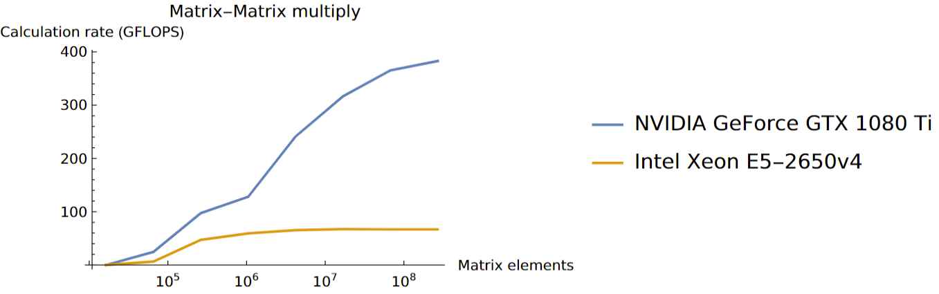
    PlotLabel -> "Matrix-Matrix multiply",
    PlotLegends -> {CUDAInformation[1,"Name"], "Intel Xeon E5-2650v4"}]]

#!/bin/bash
#SBATCH --account=<Your JGU-Account>
#SBATCH --job-name=gpu_perf
#SBATCH --output=%x_%j.out
#SBATCH --error=%x_%j.err
#SBATCH --partition=m2_gpu
#SBATCH --gres=gpu:1
#SBATCH --time=0-00:10:00
#SBATCH --mem=8192
#SBATCH --ntasks=1
#SBATCH --cpus-per-task=4

module purge
module load system/CUDA
module load math/Mathematica

math -script gpu_perf.wls

You can submit the job by executing:

sbatch math_gpu_perf_job.slurm

The job will be completed after a couple of minutes and you can view the output with:

cat gpu_perf*.out

The output should resemble the following lines:

Using a NVIDIA GeForce GTX 1080 Ti
Calculating 128.x128.
Host time: 0.10501s, GFLOPS: 0.03978592514998572
GPU time: 8.46959s, GFLOPS: 0.0004932847989099827
Calculating 256.x256.
Host time: 0.005196s, GFLOPS: 6.445130100076983
GPU time: 0.001368s, GFLOPS: 24.480187134502923
Calculating 512.x512.
Host time: 0.005688s, GFLOPS: 47.14720675105485
GPU time: 0.002756s, GFLOPS: 97.30526560232221
Calculating 1024.x1024.
Host time: 0.036191s, GFLOPS: 59.308531734409115
GPU time: 0.016779s, GFLOPS: 127.92389725251805
Calculating 2048.x2048.
Host time: 0.263092s, GFLOPS: 65.28391163547353
GPU time: 0.071256s, GFLOPS: 241.04180532165714
Calculating 4096.x4096.
Host time: 2.04433s, GFLOPS: 67.22113174291823
GPU time: 0.434158s, GFLOPS: 316.52572624712667
Calculating 8192.x8192.
Host time: 16.447865s, GFLOPS: 66.84420858950388
GPU time: 3.009729s, GFLOPS: 365.2968486239127
Calculating 16384.x16384.
Host time: 131.675999s, GFLOPS: 66.79899642722286
GPU time: 22.974397s, GFLOPS: 382.85333829445017

The graphic generated in the script is shown below: